Chain Rule for Fully Connected Neural Networks

Chain Rule for Fully Connected Neural Networks

Hello everyone! As I promised, I am publishing the first article about the chain rule for a fully connected neural network.

First, I will explain the basics of the feedforward step for a fully connected neural network, then I will derive the vector formulation backpropagation (up until last week I was considering to publish the python implementation but for backprop but for the sake of generality I will refrain from going into coding details).

First of all, some math. In this blog I will use the denominator layout notation. It means that the vectors will be treated as row vectors. This affects what the equations look like and may cause some confusion at the beginning, but it won’t be a big problem once the reader gets used to it.

1. Notation

All lower-case letters will indicate scalars/vectors whereas uppercase letters will indicate matrices.

Training a neural network consists of two steps: the forward step and the backpropagation.
First, let’s take a look at the picture below.

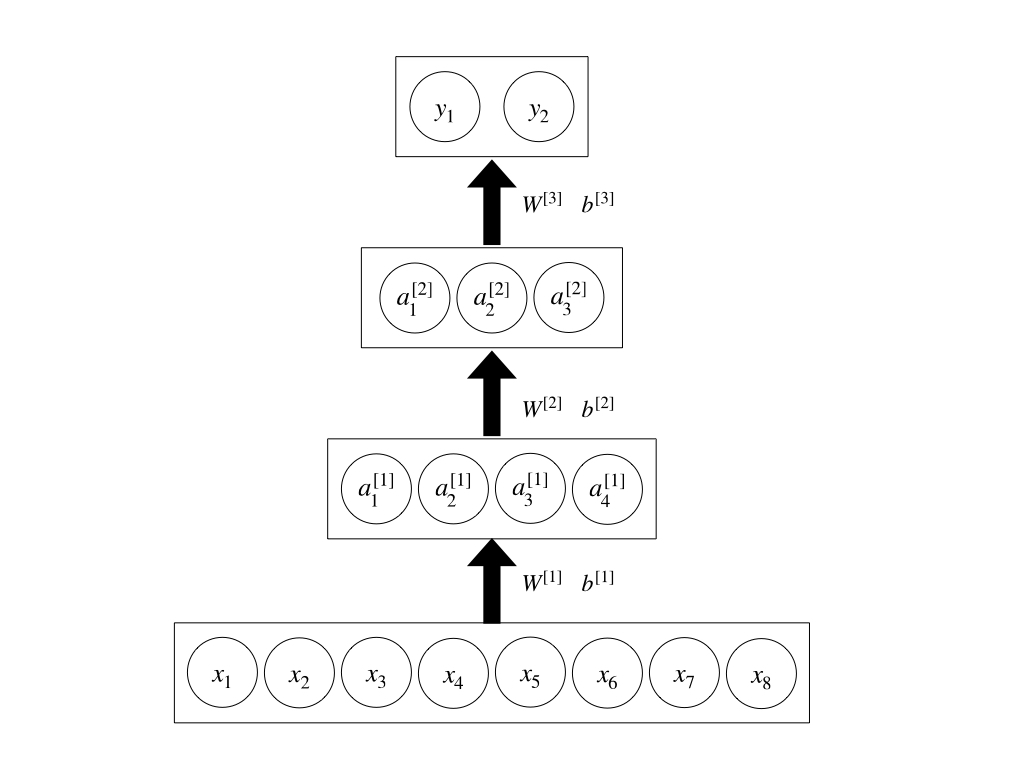
The picture above shows a fully connected neural network with 2 hidden layers, an input layer with 8 units and an output layer with 2 units. For simplicity, we will assume that the activation functions of each layer are of sigmoid type, where sigmoid $\sigma$ is:

$\begin{align*} \sigma=\frac{1}{1+e^{-x}} \end{align*}$

The forward step follows the following equations:

$z^{[1]}=xW^{[1]}+b^{[1]}$
$a^{[1]}=\sigma(z^{[1]})$
$z^{[2]}=a^{[1]}W^{[2]}+b^{[2]}$
$a^{[2]}=\sigma(z^{[2]})$
$z^{[3]}=a^{[2]}W^{[3]}+b^{[3]}$
$y=\sigma(z^{[3]})$

with:

$x \in \mathcal{R}^{(1,8)}$
$W^{[1]} \in \mathcal{R}^{(8,4)}$
$b^{[1]} \in \mathcal{R}^{(1,4)}$
$z^{[1]} \in \mathcal{R}^{(1,4)}$
$a^{[1]} \in \mathcal{R}^{(1,4)}$
$W^{[2]} \in \mathcal{R}^{(4,3)}$
$b^{[2]} \in \mathcal{R}^{(1,3)}$
$z^{[2]} \in \mathcal{R}^{(1,3)}$
$a^{[2]} \in \mathcal{R}^{(1,3)}$
$W^{[3]} \in \mathcal{R}^{(3,2)}$
$b^{[3]} \in \mathcal{R}^{(1,2)}$
$z^{[3]} \in \mathcal{R}^{(1,2)}$
$y \in \mathcal{R}^{(1,2)}$

Keep in mind that the vector-matrix multiplication gives, as outcome, another vector having as many column as the matrix.

2. Backpropagation

Before proceeding with the training, we need to define a loss function, calculate the derivative of the sigmoid and provide a two properties of matrix calculus which will be useful when calculating the derivatives.

2.1 Loss Function

The most common loss function for a neural network are the MSE-Loss (Mean Squared Error) and Crossentropy-Loss. The former is generally used on regression problems, the latter is more commonly found in classification problems.
In this article, we will consider a MSE-Loss, written as:

$E=\frac{1}{2m}\sum_{i=1}^m (g - y)^2$

The single example leads to the following error:

$E=\frac{1}{2}(g_k - y_k)^2$

Where $g$ is the ground truth and $y$ is the predicted value.

2.2 Derivative of the Sigmoid

The sigmoid has been defined above. However, during the backpropagation step we will have to use its derivative, which I will show here:

$\frac{d}{dx}\sigma(x)=\frac{d}{dx}\frac{1}{1+e^{-x}}=\frac{e^{-x}}{(1+e^{-x})^2}=\sigma(x) \frac{e^{-x}}{1+e^{-x}} = \sigma(x) \frac{1-1+e^{-x}}{1+e^{-x}}=\sigma(x) (1-\sigma(x))$

2.3 Note on matrix calculus

It is hard to find resources explaining matrix calculus in detail. A couple months ago, I found this ebook that was quite clarifying: “The matrix Cookbook”.
The hardest of backpropagation is deriving with respect to the weights. It is important to keep in mind that what I am about to state applies only to the denominator layout formulation of the neural network. If you use a numerator layout, you will need to work on the transpose to make the dimensions match.

2.3.1 The Rules

Given a product aX where a is a vector and X is a matrix, its derivatives are:

$\frac{d}{da}(aX)=X^T$

$\frac{d}{dX}(aX)=a^T$

Keep in mind that when the two rules above are applied to the chain rule in the neural network, $a^T$ has to be first term of the chain and $X^T$ has to be the last.

2.4 The backpropagation process

We need to update the matrices $W^{[1]}$, $W^{[2]}$, $W^{[3]}$ as well as the vectors $b^{[1]}$,$b^{[2]}$,$b^{[3]}$. The optimization is performed with gradient descent, therefore we need to find the following gradients:

$\frac{dE}{dW^{[1]}},\frac{dE}{dW^{[2]}},\frac{dE}{dW^{[3]}},\frac{dE}{db^{[1]}},\frac{dE}{db^{[2]}},\frac{dE}{db^{[3]}}$

Now, I have re-written the neural network above explicitly showing the output of the layer ($z^{[k]}$) before the application of the activation function.
Let’s start from $\frac{\partial E}{\partial W^{[3]}}$. The application of the chain rule allows to write the derivative as a multiplication of simpler derivatives as stated below:

$\frac{\partial E}{\partial W^{[3]}}=\frac{\partial z^{[3]}}{\partial W^{[3]}}\frac{\partial y}{\partial z^{[3]}}\frac{\partial E}{\partial y}$

The other gradients follow the same rules. Also, since the gradients with respect to $b$ are a lot easier to calculate, I will skip them in this explanation. (Consider that if you use batch normalization, $b$ does not even need to be calculated).

$\frac{\partial E}{\partial W^{[2]}}=\frac{\partial z^{[2]}}{\partial W^{[2]}}\frac{\partial a^{[2]}}{\partial z^{[2]}}\frac{\partial z^{[3]}}{\partial a^{[2]}}\frac{\partial y}{\partial z^{[3]}}\frac{\partial E}{\partial y}$

$\frac{\partial E}{\partial W^{[1]}}=\frac{\partial z^{[1]}}{\partial W^{[1]}}\frac{\partial a^{[1]}}{\partial z^{[1]}}\frac{\partial z^{[2]}}{\partial a^{[1]}}\frac{\partial a^{[2]}}{\partial z^{[2]}}\frac{\partial z^{[3]}}{\partial a^{[2]}}\frac{\partial y}{\partial z^{[3]}}\frac{\partial E}{\partial y}$

You can easily see that the many of factors composing the gradients are shared. Let’s start calculating the single terms.

For the derivative of the error with respect to the example, you need to consider the single example error and differentiate with respect to the example.

$\frac{\partial E}{\partial y}=-(g-y)$

The derivative of the example with respect to the unactivated output is given by the derivative of the sigmoid, therefore:

$\frac{\partial y}{\partial z^{[3]}}=y(1-y)$

The derivative of the unactivated output with respect to the weight matrix $W^{[3]}$ is:

$\frac{\partial z^{[3]}}{\partial W^{[3]}}={a^{[2]}}^T$ $\frac{\partial E}{\partial W^{[3]}}=-{a^{[2]}}^T \times y(1-y)(g-y)$

Where the $\times$ symbol is used to indicate the matrix multiplication. Please note that where the multiplication symbol is implied, the operation is executed elementwise. As a result:

$\frac{\partial E}{\partial W^{[3]}}=-{a^{[2]}}^T\times y(1-y)(g-y)$

Therefore $\frac{\partial E}{\partial W^{[3]}}$ is a (3,2) matrix, which is exactly the same size of $W^{[3]}$.

$\frac{\partial z^{[3]}}{\partial a^{[2]}}={W^{[3]}}^T$ $\frac{\partial a^{[2]}}{\partial z^{[2]}}=a^{[2]}(1-a^{[2]})$ $\frac{\partial z^{[2]}}{\partial W^{[2]}}={a^{[1]}}^T$

We can now build the gradient with respect to the weight matrix $W^{[2]}$. Please note that the matrix multiplication involving the weight matrix becomes the last operation in the chain rule (it is the last factor of the chain).

$\frac{\partial E}{\partial W^{[2]}}= {a^{[1]}}^T \times \left[ a^{[2]}(1-a^{[2]})\left( y(1-y)(g-y)\times {W^{[3]}}^T \right) \right]$

Therefore $\frac{\partial E}{\partial W^{[2]}}$ is a (4,3) matrix, which is exactly the same size of $W^{[2]}$.

The last derivative is the derivative of the error with respect to $W^{[1]}$

$\frac{\partial z^{[2]}}{\partial a^{[1]}}={W^{[2]}}^T$ $\frac{\partial a^{[1]}}{\partial z^{[1]}}=a^{[1]}(1-a^{[1]})$ $\frac{\partial z^{[1]}}{\partial W^{[1]}}=x^T$

Building the gradient of the error with respect to the weight matrix $W^{[1]}$ leads to:

$\frac{\partial E}{\partial W^{[1]}}= x^T\times a^{[1]}(1-a^{[1]}) \left[ a^{[2]}(1-a^{[2]})\left( y(1-y)(g-y) \times {W^{[3]}}^T \right)\right] \times {W^{[2]}}^T$

Therefore $\frac{\partial E}{\partial W^{[1]}}$ is a (8,4) matrix, which is exactly the same size of $W^{[1]}$.

Once you have calculated the previous gradients, the sum of all of them upon all the training examples will provide the accumulated gradient $\Delta W^{k}$. You can then use the $\Delta W^{k}$ to update weights and re-iterate through multiple epochs to train the network.

$W^{[1]}=W^{[1]}-\alpha \Delta W^{[1]}$
$W^{[2]}=W^{[2]}-\alpha \Delta W^{[2]}$
$W^{[3]}=W^{[3]}-\alpha \Delta W^{[3]}$

Where $alpha$ represents the chosen learning rate.

Conclusion

I have tried to explain the math behind the training of a fully connected neural network through an example. You can try to code the algorithm in numpy: it will help you cement the logic behind the neural network training.
It is true that these days we have multiple deep learning software (like Pytorch and Tensorflow) which can do the dirty job for us, but we cannot and should not forget the basics. Here you can find a link to an article by Andrej Karpathy which I recommend you to read.
Thank you for reading to the very end!